How to derive an EM algorithm from scratch
From theory to implementation
Expectation-maximization (EM) is a powerful class of statistical algorithms for performing inference in the presence of latent (unobserved) variables. There are many variations of EM being applied to solve different problems (e.g. Gaussian mixtures, HMMs, LDA, you name it). However, it is often unclear how to derive an EM algorithm, from scratch, for a new problem. In this tutorial, we will first derive and prove the general EM framework, which reveals the fundamental principles that all EM algorithms share. Then, we will use an example (mixture of exponentials) to illustrate how to derive a specific EM algorithm using this general framework for any problem.
The motivation behind EM
Maximum likelihood estimation (MLE) is a widely used parameter estimation technique in statistical inference. MLE is relatively straightforward to perform in the settings of complete observations. However, in practice, we frequently have to account for unobserved variables/parameters in the model, which we call latent variables. In these cases, the likelihood of our (observed) data actually depends on the values of the latent variables.
Formally, let $x = {x_1, x_2, \ldots}$ be the set of observed data and $z = {z_1, z_2, \ldots}$ be the (unobserved) latent variables. Let $\theta$ be the parameter that we wish to estimate and assume each $z_i \in \mathcal{Z}$ is discrete. To find the MLE of $\theta$, we need to maximize the log marginal likelihood of the data:
\[l(\theta) = \log p(x|\theta) = \log \Big(\sum_{z\in\mathcal{Z}^n} p(x, z|\theta) \Big) = \log \Big(\sum_{z\in\mathcal{Z}^n} p(x|z,\theta)p(z|\theta) \Big)\]which is often intractable (since the space of all possible combinations of $z$ can be immense) or has no closed-form solution (since we have a summation inside a log, which makes partial derivatives with respect to $\theta$ difficult).
Note that we can always treat the likelihood as a generic objective function and apply different numerical optimization techniques. EM is an iterative algorithm that solves this optimization problem faster by exploiting the probabilistic structure of the data generation process.
The general EM framework
Since all EM algorithms are just specific realizations of the general EM algorithm, we will first derive the general EM framework on the most abstract level (also from scratch!).
Derivation
The key idea behind EM is that although there is no easy way to optimize the marginal log-likelihood $l(\theta)=\log p(x|\theta)$ directly, we can construct a lower bound of it that we can easily optimize. Let $q$ be any valid distribution function for $z$,
\[\begin{align*} l(\theta) = \log p(x|\theta) &= \log \sum_{z \in \mathcal{Z}^n} p(x,z|\theta) \\ &= \log \sum_{z \in \mathcal{Z}^n} q(z)\frac{ p(x,z|\theta)}{q(z)} \\ &= \log E_{q(z)}\Big[\frac{ p(x,z|\theta)}{q(z)} \Big] \\ &\geq E_{q(z)}\Big[\log \frac{p(x,z|\theta)}{q(z)} \Big] \\ &= E_{q(z)} [\log p(x,z|\theta)] - E_{q(z)}[\log q(z)] \\ &= E_{q(z)} [\log p(x,z|\theta)] + H(q) \\ &\equiv \text{ELBO}(\theta, q) \end{align*}\]In the fourth step we applied Jensen’s inequality (and the fact that log is a concave function). You may recognize that this is exactly the Evidence Lower Bound (ELBO). Here “evidence” refers to the observed data, and it is called the ELBO because it’s a lower bound. Note that the ELBO depends on two things: the unknown parameter $\theta$ and the distribution function for the latent variable $q(z)$. Now, EM arises from the following two insights.
First, for a given $q(z)$, finding the $\theta$ that maximizes the ELBO is much easier than optimizing marginal likelihood. Let’s call the first component of this lower bound
\[Q(\theta) = E_{q(z)} [\log p(x,z|\theta)] = \sum_{z\in\mathcal{Z}^n} q(z) \log p(x,z|\theta)\]Since the second term $H(q)$ (the entropy of function $q$) does not depend on $\theta$, maximizing $Q(\theta)$ sufficient to maximize the ELBO. Notice that now the log is inside the sum, and taking derivatives with respect to $\theta$ is much easier! For this reason, we can often find analytical solutions for maximizing the ELBO as a function of $\theta$.
Second, given a fixed $\theta$, finding the $q(z)$ that maximizes the ELBO is also easy. To see this, let’s rewrite the ELBO in a different form:
\[\begin{align*} \text{ELBO}(\theta, q) &= E_{q(z)}\Big[\log \Big( \frac{p(x,z|\theta)}{q(z)} \Big) \Big] \\ &= E_{q(z)}\Big[\log \Big( \frac{p(x,z|\theta)}{p(z|x,\theta)} \frac{p(z|x,\theta)}{q(z)} \Big) \Big] \\ &= E_{q(z)}\Big[\log \Big( \frac{p(z|x,\theta)p(x|\theta)}{p(z|x,\theta)} \frac{p(z|x,\theta)}{q(z)} \Big)\Big] \\ &= E_{q(z)}\Big[\log \Big( p(x|\theta) \frac{p(z|x,\theta)}{q(z)} \Big)\Big] \\ &= E_{q(z)}[\log p(x|\theta)] - E_{q(z)}\Big[\log\Big( \frac{q(z)}{p(z|x,\theta)} \Big)\Big] \\ &= \log p(x|\theta) - \text{KL}(q || p(z|x,\theta)) \end{align*}\]Here we can see that the gap between the ELBO and the marginal log-likelihood is exactly the Kullback–Leibler (KL) divergence between $q$ and $p(z|x,\theta)$, a.k.a the posterior of the latent variable conditioned on the observed data and the parameter $\theta$. Since KL between two distributions is non-negative and is only 0 when they are exactly the same, it becomes apparent that the choice of $q(z)$ that maximizes the ELBO is precisely $p(z|x,\theta)$.
Combining the above two observations, we arrive at an iterative procedure to obtain ML estimate of $\theta$, which alternates between optimizing the ELBO with respect to $\theta$ while holding $q(z)$ fixed, then with respect to $q(z)$ while holding $\theta$ fixed.
- Initialize $\theta = \theta^{(0)}$.
- (E-step) Compute the posterior of the latent variables $p(z | x,\theta^{(t)})$ and use it to compute $Q(\theta)$.
- (M-step) Find new $\theta$ estimate that maximizes $Q(\theta)$; i.e., $\theta^{(t+1)} = \arg \max_\theta Q(\theta)$.
The second step is called the E-step because it involves the computation of $Q$, which is an expectation. The third step is called the M-step because it is maximizing the objective function $Q(\theta)$. Note that $Q$ can be viewed as the same function across time steps but configured with different $\theta^{(t)}$s, so we often write it as $Q(\theta; \theta^{(t)})$, a function of both $\theta$ and $\theta^{(t)}$.
The E-step is in some way also a maximization step, because choosing $q(z) = p(z | x,\theta^{(t)})$ maximizes the ELBO at $\theta = \theta^{(t)}$ (in fact, it is exactly equal to $l(\theta^{(t)})$, the log marginal likelihood at $\theta = \theta^{(t)}$). In this way, EM can be viewed as a special case of coordinate ascent.
Visualization
Here is a graphical illustration of how the iterative update works:
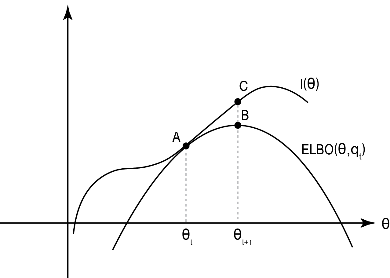
Figure 1. EM parameter update at iteration $t$. Two functions are plotted: the log marginal likelihood $l(\theta)$ and the ELBO computed using $q_t(z)=p(z|x,\theta^{(t)})$. The gap between $l(\theta)$ and the ELBO is the KL divergence between $q_t(z)$ and $p(z|x;\theta)$. In the M-step, we move from point A to point B by optimizing ELBO with respect to $\theta$. In the E-step, we maximize the ELBO at the updated $\theta$ by updating the $q(z)$ function, moving from point B to point C.
Proof of correctness
How do we know whether EM is guaranteed to converge? It can be proved that the marginal likelihood monotonically increases with each parameter update. i.e.,
\[l(\theta^{(0)}) \leq l(\theta^{(1)}) \leq l(\theta^{(2)}) \leq \cdots\]From the diagram above, we can intuitively see why this is true. The three points that we have marked on the graph respectively represent three key quantities:
\[\begin{align*} A&: \text{ELBO}(\theta^{(t)},q_t)=l(\theta^{(t)}) \\ B&: \text{ELBO}(\theta^{(t+1)},q_t) \\ C&: l(\theta^{(t+1)}) \end{align*}\]Intuitively, B is always higher than A, and C is always higher than B in the graph. More formally,
\[l(\theta^{(t+1)}) \geq \text{ELBO}(\theta^{(t+1)},q_t) \geq \text{ELBO}(\theta^{(t)},q_t)=l(\theta^{(t)})\]Where the first inequality is because ELBO is always a lower bound of $l$, the second is because we choose the new $\theta$ to be the maximizer of the current ELBO, and the final inequality is that $q_t$ was chosen so that the current ELBO is exactly equal to $l$ at the current $\theta$. Therefore, each time we update $\theta$ (M-step) we attain a higher marginal likelihood.
On the other hand, when we update $q(z)$ while keeping $\theta$ fixed (E-step), we choose $q_{t+1}$ such that we make the ELBO exactly equal to $l$ at the current $\theta$. So,
\[\text{ELBO}(\theta^{(t)},q_{t+1}) = l(\theta^{(t)}) \geq \text{ELBO}(\theta^{(t)},q_t)\]so each time we update $q(z)$ we make the ELBO a tighter bound of $l$ at the current $\theta$.
We can now appreciate that with a few lines of derivations, we have achieved something significant: we have derived and proved a general class of EM algorithms that can be applied to a wide range of statistical models.
Deriving an EM algorithm
General procedure
Based on the framework above, we have the following steps for deriving the EM update rules for specific inference problem. To be more general, let’s use $\Theta$ to denote the collection of parameters in a model.
- To derive the E-step (finding the lower bound), write down the conditional posterior $p(z|x,\Theta^{(t)})$ and the $Q(\Theta; \Theta^{(t)})$ function:
- To drive the M-step (updating parameters to maximize the lower bound), find an analytical formula for $\Theta$ such that \(\Theta^{(t+1)} = \arg\max_\Theta Q(\Theta; \Theta^{(t)})\)
This gives the parameter update rule.
Example derivation
Let’s go over a concrete example to see how EM derivation works in action. Let’s say we are trying to infer the failure rates of light bulbs coming from different manufacturing batches. Let $x_i$ be the observed failure time of lightbulb $i \in {1\ldots n}$, and $z_i \in {1, \ldots, K}$ be the batch that lightbulb $i$ came from (which we do not observe). Let’s model the failure time using an exponential distribution, where the failure rate is different for each batch $k$:
\[x_i |z_i = k \overset{ind}{\sim} \text{Expo}(\lambda_k)\]The batch itself is drawn from a categorial distribution:
\[z_i \overset{i.i.d.}{\sim} \text{Categorical}(\pmb{\pi})\]To make the problem more challenging, let’s say both $\pmb{\lambda} = (\lambda_1, \lambda_2, \ldots, \lambda_K)$ and $\pmb{\pi} = (\pi_1, \pi_2, \ldots, \pi_K)$ are unknown. Let’s denote the collection of these model parameters as $\Theta = (\pmb{\lambda}, \pmb{\pi})$. Well, how do we figure out the failure rates of different light bulb batches, if the batch labels themselves are unknown? Let’s see how we can derive an EM algorithms that can achieve this.
First, let’s derive the E-step.
\[\begin{align*} Q(\Theta; \Theta^{(t)}) &= E_{z} [\sum_i \log p(x_i,z_i|\Theta)] \\ &= \sum_i E_{z} [\log p(x_i|z_i,\pmb{\lambda}) p(z_i|\pmb{\pi})] \\ &= \sum_i \{ E_{z} [\log p(x_i|z_i,\pmb{\lambda})] + E_z[ \log p(z_i|\pmb{\pi})] \} \end{align*}\]We can see that the $Q$ function is broken up into two main components, which are respectively:
\[\begin{align*} \sum_i E_{z} [\log p(x_i|z_i,\pmb{\lambda})] &= \sum_i \sum_k p(z_i=k|x_i,\Theta^{(t)}) \log p(x_i|z_i=k,\lambda_k) \\ &= \sum_i \sum_k \phi^t_{z_i}(k) (\log \lambda_k - \lambda_k x_i) \end{align*}\] \[\begin{align*} \sum_i E_z[ \log p(z_i|\pmb{\pi})] &= \sum_i \sum_k p(z_i=k|x_i,\Theta^{(t)}) \log \pi_k \\ &= \sum_i \sum_k \phi^t_{z_i}(k) \log \pi_k \end{align*}\]Where we have defined $\phi^t_{z_i}(k) = p(z_i=k|x_i,\Theta^{(t)})$, which is intuitively the membership probability that lightbulb $x_i$ belongs to batch $k$. Note that this quantity does not dependent on $\Theta$ (it only depends on $\Theta^{(t)}$, which is treated as a known constant). Also, $\sum_k \phi^t_{z_i}(k) = 1$ since it is a conditional probability. We can compute it using Bayes’ Rule:
\[\begin{align*} \phi^t_{z_i}(k) &= p(z_i=k|x_i,\Theta^{(t)}) \\ &= \frac{p(x_i|z_i=k,\lambda^t_k)p(z_i = k|\pi^t_k)}{\sum_k p(x_i|z_i=k,\lambda^t_k)p(z_i = k|\pi^t_k)} \\ &= \frac{\lambda_k^t \text{exp}(-\lambda_k^t x_i) \pi_k^t}{\sum_k \lambda_k^t \text{exp}(-\lambda_k^t x_i) \pi_k^t} \end{align*}\]All together, we have
\[Q^t(\Theta) = \sum_i \sum_k \phi^t_{z_i}(k) (\log \lambda_k - \lambda_k x_i) + \sum_i \sum_k \phi^t_{z_i}(k) \log \pi_k\]which is a function of $\pmb{\lambda},\pmb{\pi}$ and $\pmb{\lambda}^{(t)},\pmb{\pi}^{(t)}$.
Now, let’s derive the M-step. Taking partial derivatives with respect to each $\pi_k$ parameter, while adding a Lagrange multiplier $\alpha$ for the constraint $\sum_k \pi_k = 1$, we have:
\[\frac{\partial (Q^t + \alpha(1-\sum_k \pi_k))}{\partial \pi_k} = \sum_i \frac{\phi^t_{z_i}(k)}{\pi_k} - \alpha \overset{\Delta}{=} 0 \\ \implies \pi_k = \frac{\sum_i \phi^t_{z_i}(k)}{\alpha}\]Since $\sum_k \pi_k = 1$ and $\phi^t_{z_i}(k) = 1$,
\[\begin{align*} \frac{\sum_k \sum_i \phi^t_{z_i}(k)}{\alpha} &= 1 \\ \alpha &= \sum_i \sum_k \phi^t_{z_i}(k) = \sum_i 1 = n \end{align*}\]So this means that the parameter update for $\pi_k$ is
\[\pi_k = \frac{\sum_i \phi^t_{z_i}(k)}{n}\]For $\lambda_k$, take partial derivative again:
\[\frac{\partial Q^t}{\partial \lambda_k} = \sum_i \phi^t_{z_i}(k) (\lambda_k^{-1}-x_i) \overset{\Delta}{=} 0 \\ \implies \lambda_k = \frac{\sum_i \phi^t_{z_i}(k) }{\sum_i \phi^t_{z_i}(k)x_i }\]Putting the two steps together, we have the following iterative update rules:
- Initialize $\pi^{(0)}_k = 1/K$ and $\lambda^{(0)}_k = 1$.
- (E-step) Compute $\phi^t_{z_i}(k)$ and $Q^t(\Theta)$, where
- (M-step) Update parameters
which works for any exponential mixtures. Note that the $Q$ function does not need to be explicitly computed, because we have an analytical solution for maximizing it (which is our M-step).
Implementation
Here is an implementation of the EM algorithm we just derived (in R).
library(dplyr)

get_phi_k = function(k, lambda_t, pi_t, x_i) {
    l = sapply(1:K, function(k){
        lambda_t[k] * exp(-lambda_t[k] * x_i) * pi_t[k]
    })
    phi_k = l[k]/sum(l)
    return(phi_k)
}

update_lambda_k = function(k, phi_k, x) {
    lambda_k = sum(phi_k)/sum(phi_k*x)
    return(lambda_k)
}

update_pi_k = function(k, phi_k) {
    pi_k = sum(phi_k)/N
    return(pi_k)
}

run_em = function(x, max_iter = 10) {

    # initialization
    pi = list()
    lambda = list()
    pi[[1]] = rep(1/K, K)
    lambda[[1]] = 1:K

    for (t in 1:(max_iter-1)) {

        # E-step
        phi = lapply(1:K, function(k) {
            sapply(1:N, function(i) {
                get_phi_k(k, lambda[[t]], pi[[t]], x[i])
            })
        })

        # M-step
        lambda[[t+1]] = sapply(1:K, function(k) {
            update_lambda_k(k, phi[[k]], x)
        })

        pi[[t+1]] = sapply(1:K, function(k) {
            update_pi_k(k, phi[[k]])
        })

    }

    return(list(lambda = lambda, pi = pi))
}
Let’s simulate some data, with 3 batches each with different failure rates.
K = 3
N = 1000
set.seed(2)

x = c(
    rgamma(n = 500, shape = 1, rate = 1),
    rgamma(n = 300, shape = 1, rate = 10),
    rgamma(n = 200, shape = 1, rate = 100)
) %>% sort

n_iter = 100
res = run_em(x, max_iter = n_iter)
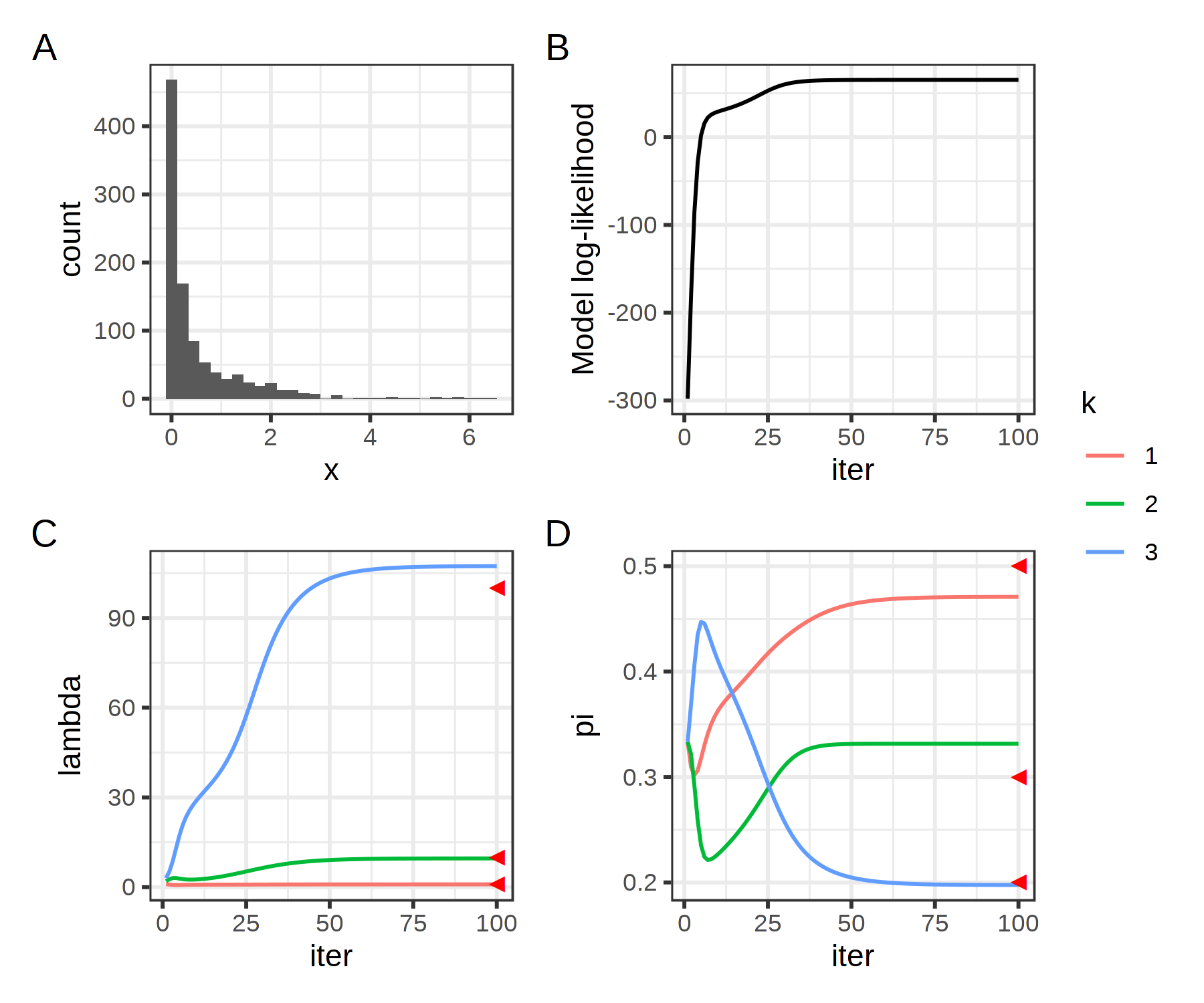
Figure 2. A, Distribution of the simulated data. B, log-model likelihood across iterations. C and D, parameter estimates at each iteration. Red triangles mark the true parameter values.
We see that the algorithm converges after 50 iterations or so, with monotonically improving model fit. Even though we can’t spot any obvious batch effects in the distribution of the data, the failure rate and prevalence of each batch estimated by EM are pretty much spot-on!
Acknowledgements
Thanks to Hirak Sarkar for providing helpful feedback. The illustration in Figure 1 was largely inspired by this post.